J Korean Soc Magn Reson Med.  2014 Jun;18(2):107-119. 10.13104/jksmrm.2014.18.2.107.

A Tool Box to Evaluate the Phased Array Coil Performance Using Retrospective 3D Coil Modeling

• Perez M
• Hernandez
• Michel E
• Cho MH
• Lee SY

• KMID: 2099887
• DOI: http://doi.org/10.13104/jksmrm.2014.18.2.107

Abstract

PURPOSE
To efficiently evaluate phased array coil performance using a software tool box with which we can make visual comparison of the sensitivity of every coil element between the real experiment and EM simulation.
MATERIALS AND METHODS
We have developed a C++- and MATLAB-based software tool called Phased Array Coil Evaluator (PACE). PACE has the following functions: Building 3D models of the coil elements, importing the FDTD simulation results, and visualizing the coil sensitivity of each coil element on the ordinary Cartesian coordinate and the relative coil position coordinate. To build a 3D model of the phased array coil, we used an electromagnetic 3D tracker in a stylus form. After making the 3D model, we imported the 3D model into the FDTD electromagnetic field simulation tool.
RESULTS
An accurate comparison between the coil sensitivity simulation and real experiment on the tool box platform has been made through fine matching of the simulation and real experiment with aids of the 3D tracker. In the simulation and experiment, we used a 36-channel helmet-style phased array coil. At the 3D MRI data acquisition using the spoiled gradient echo sequence, we used the uniform cylindrical phantom that had the same geometry as the one in the FDTD simulation. In the tool box, we can conveniently choose the coil element of interest and we can compare the coil sensitivities element-by-element of the phased array coil.
CONCLUSION
We expect the tool box can be greatly used for developing phased array coils of new geometry or for periodic maintenance of phased array coils in a more accurate and consistent manner.

Keyword

Phase array coil; Performance evaluation; 3D modeling; FDTD; 3D tracker

MeSH Terms

Electromagnetic Fields
Magnetic Resonance Imaging
Magnets
Retrospective Studies*

Figure

• 

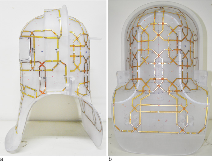
  Fig. 1 A physical phased array 36 channel helmet-style coil structure. (a) Lateral view and (b) frontal view of the 36-ch passed array coil structure.

• 

  Fig. 2 Data acquisition protocol and PACE tool box.

• 

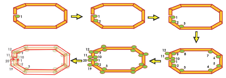
  Fig. 3 Representation of the pinpointed landmarks (green circles) obtained by the 3D tracker of the FASTSCAN to define the coil element geometry. Starting at the upper-left figure: The first landmark acquired, second landmark, etc. Bottom-left: All the landmarks connected giving the periphery of the coil element.

• 

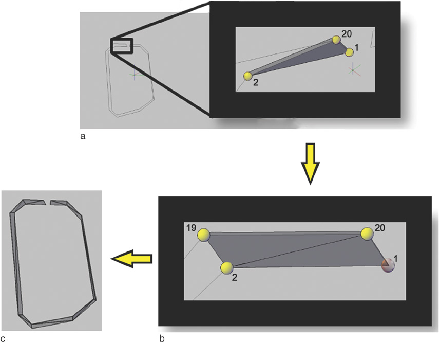
  Fig. 4 Representation of the coil element construction done in ARCS by using the 3D tracker file containing the landmarks. (a) Connection of the first three points of the first coil element at a specified thickness. (b) Second triangular prism created with the nearest neighboring point. Each coil element is completed by repeating this procedure until all the points are connected. (c) Creation of a complete coil element.

• 

  Fig. 5 Distribution of the simulated magnetic field produced by a coil element of the phased array coil. The coil model was created by AUTOCAD with the ARCS (from PACE toolbox) script, while the FDTD evaluation was done in SEMCAD X. (a) YZ plane, (b) XY plane, and (c) XZ plane. The signal was normalized to 0.000498 Vs/m^2.

• 

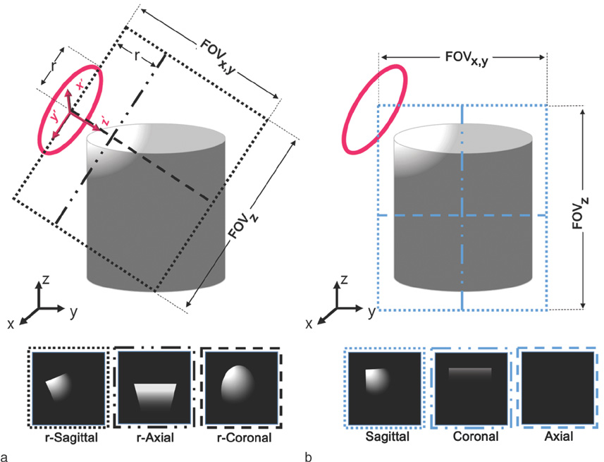
  Fig. 6 Representation of the rotated Cartesian coordinate relative to the coil plane and the traditional one. (a) The rotated Cartesian coordinate should meets the highest signal from a well decoupled element on a phase array coil. The rotated z-axis points perpendicularly to the center of the coil element plane. (b) Traditional Cartesian coordinate visualization planes at x=0, y=0 and z=0 will not fully represent the sensitivity of a well decoupled and localized coil element.

• 

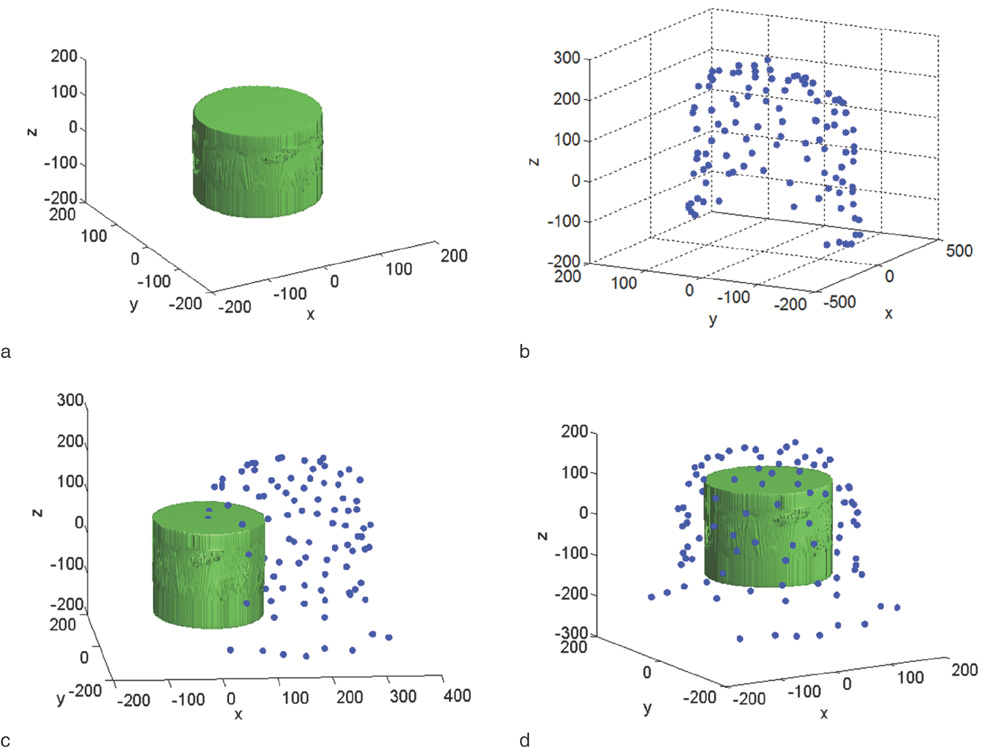
  Fig. 7 Representation of co-registration process of the coil structure points and the acquired volume sensitivity map. (a) Isosurface of the Sum-of-Square (SoS) from the experimental data in mm. (b) Points representing each coil element in mm. (c) Both set of data located in different coordinate systems. (d) Both set of data after co-registration.

• 

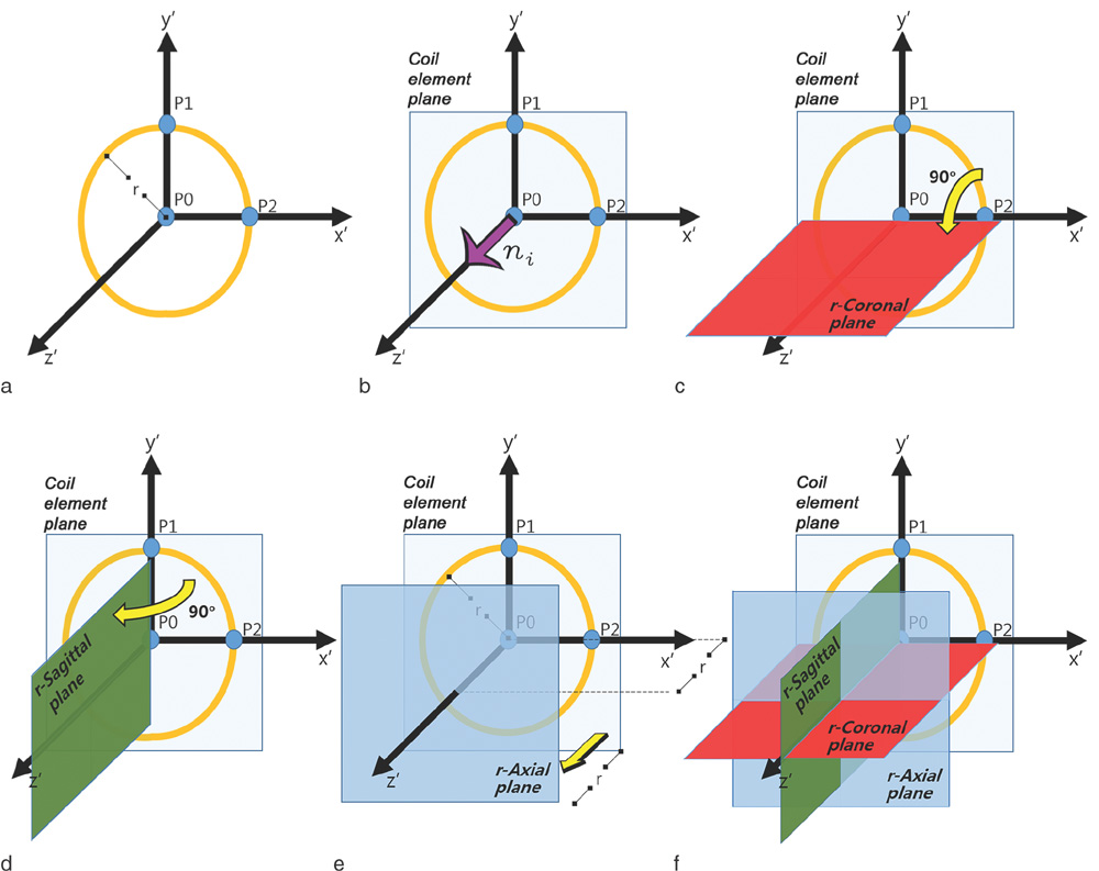
  Fig. 8 Representation of the relative-planes creation. (a) Three points (Coil element plane points) representing each coil element. (b) Computed coil element plane using Eq. 2. (c) The r-Coronal plane generated by rotating 90° the coil element plane with an axis rotation along x'. (d) The r-Sagittal plane generated by rotating 90° the coil element plane with an axis rotation along y'. Equation 4 was used in (c) and (d) cases. (e) The r-Axial plane generated using Eq. 3, the coil element plane shifted to a distance given by the radius of the coil element. (f) The three relative-planes and coil element plane positions.

• 

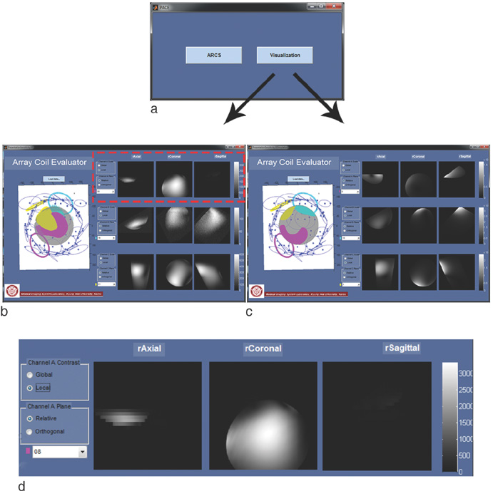
  Fig. 9 The MATLAB-based PACE toolbox visualization software comparing the sensitivities of the coil elements between the real MRI experiment and the expected performance through the FDTD simulation. (a) Main PACE window where is possible to choose ARCS or the visualization window. (b) MRI experiment on PACE visualization window. (c) FDTD Simulation on PACE visualization window. (d) Zoom from the dotted box on (b). (b) and (c) shows coils #8, #19 and #1 from top to the bottom.

• 

  Fig. 10 SEMCAD visualization of the reconstructed 3D model of the 36 channel helmet-style coil structure shown in Fig. 1. (a) Lateral view and (b) frontal view of the 3D model. The 3D model was reconstructed by AUTOCAD using PACE tool box from the landmarks measured by the 3D tracker.

• 

  Fig. 11 Extracted figures from the MATLAB-based PACE toolbox visualization software, comparing the MRI data and the simulation sensitivities of a single coil element (channel #19) by the relative (Proposed) and Cartesian (Ordinary) views. (a) Coil structure and simulation isosurface co-registered. In magenta, the analyzed coil element with its maximum signal distribution. (b) Coil structure and MRI data isosurface co-registered. In magenta, the analyzed coil element with its maximum signal. (c-e) Cartesian -axial, -coronal and -sagittal views, respectively, from the simulation. (f-h) relative -axial, -coronal and -sagittal views, respectively, from the simulation. (i-k) Cartesian -axial, -coronal and -sagittal views, respectively, from the MRI data. (l-n) relative -axial, -coronal and -sagittal views, respectively, from the MRI data.

Reference

1. Roemer PB, Edelstein WA, Hayes CE, Souza SP, Mueller OM. The NMR phased array. Magn Reson Med. 1990; 16:192–225.

2. Lee RF, Giaquinto RO, Hardy CJ. Coupling and decoupling theory and its application to the MRI phased array. Magn Reson Med. 2002; 48:203–213.

3. Keil B, Wald LL. Massively parallel MRI detector arrays. J Magn Reson. 2013; 229:75–89.

4. Wong EY, Hillenbrand CM, Lewin JS, Duerk JL. Computer simulations for optimization of design parameters for intravascular imaging microcoil construction. Proc Intl Soc Mag Reson Med. 2003; 11:2386.

5. Constantinides C, Angeli S, Gkagkarellis S, Cofer G. Intercomparison of performance of RF coil geometries for high field mouse cardiac MRI. Concepts Magn Reson Part A Bridg Educ Res. 2011; 38A:236–252.

6. Hernandez D, Perez M, Lee SY. A bi-planar surface coil for parietal lobe imaging. Proc Intl Soc Mag Reson Med. 2013; 21:2793.

7. Kim DE, Park YM, Perez M, Hernandez D, Lee JH, Lee SY. Retrospective 3D modeling of RF coils using a 3D tracker for EM simulation. Concepts Magn Reson Part B. 2013; 43:126–132.

8. Wiggins GC, Triantafyllou C, Potthast A, Reykowski A, Nittka M, Wald LL. 32-channel 3 tesla receive-only phased-array head coil with soccer-ball element geometry. Magn Reson Med. 2006; 56:216–223.

9. Lattanzi R, Grant AK, Polimeni JR, et al. Performance evaluation of a 32-element head array with respect to the ultimate intrinsic SNR. NMR Biomed. 2010; 23:142–151.

10. Hoult DI. The principle of reciprocity in signal strength calculations-A mathematical guide. Concepts Magn Reson Part A. 2000; 12:173–187.

11. Hartwig V, Tassano S, Mattii A, et al. Computational analysis of a radiofrequency knee coil for low-field MRI using FDTD. Applied Magn Reson. 2013; 44:389–400.

12. Darrasse L, Kassab G. Quick measurement of NMR-coil sensitivity with a dual-loop probe. Review Scientific Instruments. 1993; 64:1841–1844.

13. SEMCAD X MRI. Web site. http://www.speag.com/.

14. Griswold MA, Jakob PM, Nittka M, Goldfarb JW, Haase A. Partially parallel imaging with localized sensitivities (PILS). Magn Reson Med. 2000; 44:602–609.

15. Seiberlich N, Griswold M. Parallel imaging in angiography. Magnetic Resonance Angiography. Springer;2012. p. 188.